 Order Linear with a Forcing Function
Order Linear with a Forcing Function
Order Linear with a Forcing Function
The second order linear ODE
![]()
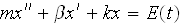 arises in many applications. Two of the more obvious are LRC circuits and
harmonic oscillators. The purpose of this lab is to illustrate the effect of
forcing functions on different linear ODE's.
arises in many applications. Two of the more obvious are LRC circuits and
harmonic oscillators. The purpose of this lab is to illustrate the effect of
forcing functions on different linear ODE's.
The first three are more prevalent in applications:
1.
![]()
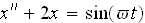 For this one we will make 4 different graphs. Using
![]()
 and
and
![]()
 make a graph for each value of
![]()
 0.5, 1.2, 1.4, 2.0. One on these will illustrate beats and another
resonance while the other two are noise, Try to decide as to which is which.
Run the t scales far enough to determine what is happening in each case.
0.5, 1.2, 1.4, 2.0. One on these will illustrate beats and another
resonance while the other two are noise, Try to decide as to which is which.
Run the t scales far enough to determine what is happening in each case.
2.
![]()
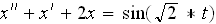 For this one we will change the initial condition,
![]()
 ,
values and graph all on the same graph. Let
,
values and graph all on the same graph. Let
![]()
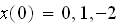 while x'(0)=0. What seems to be happening now?
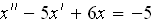
3.
![]()
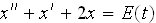 Now we change the forcing function and graph all on the same graph. For
simplicity and for clarity as to whats happening we are going to let
Now we change the forcing function and graph all on the same graph. For
simplicity and for clarity as to whats happening we are going to let
![]()
 be the constant functions
![]()
 ,
,
![]()

![]()

For 4., 5., 6. make one graph
each showing the three equations on the same field. In each case use
![]()

![]()
 and try to decide what effect the forcing function has on the graphs.
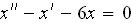
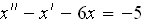
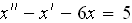
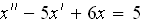
4.
![]()
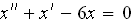 and
and
![]()
 and
and
![]()
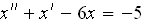
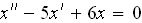
5.
![]()
 and
and
![]()
 and
and
![]()
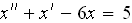
6.
![]()
 and
and
![]()
 and
and
![]()
Report your findings.
This document created by Scientific Notebook 4.1.