PHY 2425 - Engineering Physics I

Kinesthetic Kinematics

Leader: _________________________ Recorder: __________________________

Skeptic: _________________________ Encourager: ________________________

Materials

Laptop

LabPro

ULI Motion Detector with C-clamp

Introduction

The purpose of this lab is to develop an intuitive understanding of the graphs of position, velocity, and acceleration as a function of time. Once position as a function of time, x(t), is known, then all other kinematic quantities can be found. This is true since the velocity and acceleration can be found from the position from the relations v(t) = and a(t) = . Graphically, we can interpret the velocity as the slope of the position function, and similarly the acceleration gives the concavity of the position function. Thus from having the graph of the position function, we can determine the graphs of the velocity and acceleration functions. We will make use of this to produce graphs having certain properties using a sonic motion detector.

Procedure

Our procedure will be to record the position as a function of time using ourselves as the object of study. We will measure our position as a function of time using the LabPro and a sonic motion detector.

The sonic motion detector makes use of the fact that sound travels at a constant speed through the air in order to measure distances. The motion detector measures position by emitting a brief pulse of ultrasound (frequency = 40,000 Hz) towards a target and then detecting the sound reflected from the target. The detector determines the time interval between when the pulse of sound is emitted and the reflected sound returns. The distance is determined from d = v_st_r/2, where v_s is the speed of sound, and t_r is the measured time interval. The result is divided by 2 because the time interval represents a round trip for the sound, and is thus double the distance to the target. The speed of sound depends on the temperature, but at room temperature, the speed is approximately 343 m/s, and this is the value used by the motion detector in determining distances.

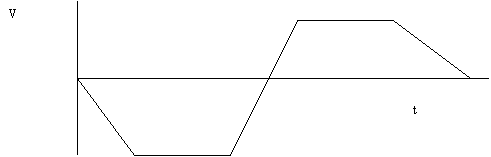
1. Set-up

The experimental set up is shown in figure 1. To set up the apparatus, plug the cable from the motion detector into the socket labeled DIG/SONIC 1 on the LabPro. Verify that the LabPro is plugged into the computer and that it has power. Clamp the motion detector to the lab table or the back of a chair in a position such that the motion detector has an unobstructed view of you walking towards and away from the it over a distance of several meters. The motion detector attaches to the clamp via a bushing on the back. Alternatively, you can just place the motion detector on the table. The motion detector can be easily secured with a piece of masking tape rolled underneath. Note that the motion detector will not allow you to measure distances of less than .4 m or greater than about 6 m.

2. Start the Software

On the task bar is an icon which looks like the jaws of a caliper. Click on the icon to launch the program called LoggerPro. Open the experiment file titled motion detector by clicking on the open icon (alternatively you can click on the File menu and then click on Open…). Double click on the folder labeled Probes and Sensors then double click on the folder labeled Motion Detector, and then finally double click on the file labeled Motion Detector.

3. Test the Set-up

To verify that the apparatus is running correctly, we will make a quick graph of position versus time. The monitor should display blank graphs of Position versus Time, velocity vs. time, and acceleration vs. time. On the right and above the graph is a small button labeled COLLECT . Click on the collect button. The motion detector should click twice, and then make a continuous clicking sound for five seconds during which it is collecting data. Move your hand back and forth in front of the motion detector and verify that it is operating correctly. If not contact your instructor.

Figure 1

Apparatus for this experiment

4. Printing

One last thing we need to do is print our graphs. Click on the Printer Button on the tool bar. You will be prompted if you wish to prompt all three windows or not. Click on YES. Then you will see a second window where you can annotate your graphs such as putting the group members’ names on them and so on. Click OK when you're ready to print.

Turn in One report with accompanying graphs and answers to questions per group. Note that in all sketches you make by hand, you should include properly labeled axes.

Now that we have got our apparatus working, we will acquire the following pictures. Follow the instructions in the order listed. When asked to make a prediction, make the prediction before carrying out the experiment. Predictions are only graded for making them and not for being correct.

I. a) First, describe in the provided space how you would move so that the position increases linearly with time. Be specific.

b) In the space below, sketch graphs of your predictions of what the graph of the position vs. time, velocity vs. time and acceleration vs. time should look like for this motion?

c) Collect data of a person in your group moving in the described manner.

d) Look at the graphs on the computer, and discuss their appearance compared to your prediction. (A sentence or so for each graph will suffice.) Note that the acceleration graph may appear very erratic. Why?

Attach one set of graphs per group consisting of position vs. time, velocity vs. time, and acceleration vs. time.

II. a) Describe in the provided space how you would move so that the position decreases linearly with time. Be specific.

b) In the space below, sketch graphs of your predictions of what the graph of the position vs. time, velocity vs. time and acceleration vs. time should look like for this motion?

c) Collect data of a person in your group moving in the described manner.

d) Look at the graphs on the computer, and discuss their appearance compared to your prediction. (A sentence or so for each graph will suffice.)

Attach one set of graphs per group consisting of position vs. time, velocity vs. time, and acceleration vs. time.

III. a) Describe in the provided space how you would move so that the position increases with time and the graph is concave up. Be specific.

b) Sketch a graph of your prediction of what the graph of the velocity vs. time should look like for this picture?

c) Sketch a graph of your prediction of what the graph of Acceleration vs. time should look like for this picture?

d) Collect data of a person in your group moving in the described manner.

e) Look at the graphs on the computer, and discuss their appearance compared to your prediction. (A sentence or so for each graph will suffice.)

Attach one set of graphs per group consisting of position vs. time, velocity vs. time, and acceleration vs. time.

IV. a) Describe in the provided space how you would move so that the position increases with time and the graph is concave down. Be specific.

b) Sketch a graph of your prediction of what the graph of Velocity vs. time should look like for this picture?

c) Sketch a graph of your prediction of what the graph of the acceleration vs. time should look like for this picture?

d) Collect data of a person in your group moving in the described manner.

e) Look at the graphs on the computer, and discuss their appearance compared to your prediction. (A sentence or so for each graph will suffice.)

Attach one set of graphs per group consisting of position vs. time, velocity vs. time, and acceleration vs. time.

V. Each person in your group should collect data and print out a graph where the position varies approximately sinusoidially in time.

a) How do you have to move in order to obtain such a graph?

On the graph mark the following:

b) each interval where the velocity is positive.

c) each interval where the velocity is negative.

d) each interval where the acceleration is positive.

e) each interval where the acceleration is negative.

Attach the Graph for each person to the report.

VI. Sketch by hand in the space below graphs of position versus time for the following types of motions.

a) The velocity and the acceleration are both zero.

b) The velocity is initially positive and the acceleration is negative.

c) The velocity is initially negative and the acceleration is positive.

d) The velocity is initially zero, but the acceleration is positive

VII. a) Describe how to construct a graph of position versus time which will at first have a constant negative velocity of -1 m/s and then will smoothly change until it has a constant positive velocity of 1 m/s.

b) Predict what the acceleration versus time graph will look like.

c) Carry out such a motion, and print the graphs.

d) On the graphs indicate the intervals where the acceleration is positive and negative.

e) On the graphs indicate the intervals where the speed is increasing and decreasing.

f) Explain why even though the acceleration is positive, over a certain interval, the speed decreases over part of the interval and increases over part of the interval.

VIII. Click on the Open icon . The Motion Detector directory should already be open. Double click on the file called Distance Match. Click on No if asked to save changes.

The computer will display a graph of distance versus time. When you hit the collect button, the graph of your motion will be shown on the same graph. Have each person in the group try to match the graph as closely as possible. Print and attach your best result.

On your printed graph indicate the following.

a) Intervals where the velocity was positive.

b) Intervals where the velocity was negative

c) Intervals where the velocity was 0.

IX. Click on the open folder icon. Double click on the file title Velocity Match, saying NO when it asks you to save changes. LoggerPro will show a graph of velocity versus time. When you click on the collect button, your velocity will be shown on the same graph. Have each person in your group try to match the graph. (This one is tricky.) Print and attach your best result. Hint: This is a graph of how fast you are moving, not where you are.

On your printed graph indicate the following.

a) Intervals where the velocity was positive.

b) Intervals where the velocity was negative

c) Intervals where the velocity was 0.

d) Intervals where you had a positive acceleration

e) Intervals where you had a negative acceleration

X. Write a story describing the motion (including direction) of a car which has a velocity versus time graph which looks like the following.