PHYS 2425 – Engineering Physics I
Air Resistance
Leader: _____________________________ Recorder:
___________________________
Skeptic: _____________________________ Encourager:
_________________________
Materials
Laptop
LabPro
Motion Detector
Coffee Filters (small basket
type)
Ring stand with right angle
and jaw clamp
Introduction
In this
lab we will investigate the effect that resistive forces have on the motion of
a falling object. A resistive force such
as air resistance depends on the velocity of the object. The simplest model for a velocity dependent
resistive force is that the force is proportional to the velocity, F(v) = -bv. The constant b
depends on the properties of the medium through which the object drops as well
as the shape and geometry of the object.
This model tends to work well for small objects moving slowly. A second and usually more realistic model
commonly used to model air resistance is the air resistance is quadratic in the
velocity. We typically write the
resistive force for the case of a quadratic model as F(v)
= - 1/2 CrAv2, where r is the density of the
medium through which the object falls, A is the cross sectional area of the
object, and C is a constant known as the drag coefficient.
Q1. Draw a
free body diagram for a falling object including air resistance.
Q2. Write
We will now analyze the behavior of the equation
qualitatively. If we drop the object
from rest, it initially has a velocity of zero, and consequently the air
resistance is zero.
Q3. How does
the magnitude of the resistance force change as the object falls?
Q4. If the
magnitude of the resistance force increases as the object falls, then what
happens to the net force on the object as it falls?
Q5. If the
net force becomes 0, the velocity becomes constant. This velocity is called the terminal velocity. Find an expression for the terminal velocity
for the case of a linear resistive force in terms of b, g, and m.
Q6. Find an
expression for the terminal velocity for the case of a quadratic resistive
force in terms of c, ρ, g, A, and m.
Q7. Compare the two expressions for the terminal
you have found. We can differentiate
them by how they depend on mass.
Describe how each expression for the terminal velocity depends on the
mass.
Procedure
We will
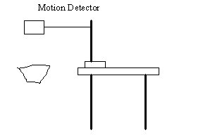
employ the motion detector to obtain data for this lab. The experimental set up is shown in figure 1.
Figure 1 Schematic of experimental set up
1. Set Up
Clamp the
motion detector so that it faces down, is level, and is as high as possible
above the floor. Connect the motion
detector to DIG/SONIC 1 of the LabPro.
We will
use as the objects to drop in this experiment stacks of various numbers of
coffee filters. These make ideal objects
for this experiment. The mass is small making
air resistance important. Also the mass can
be easily adjusted by simply adding more coffee filters to the stack while
maintaining an effectively constant cross sectional area. Start
up LoggerPro and open the experiment file titled “Motion
Detector” by following the path “Probes and Sensors”=>”Motion
Detector”=>”Motion Detector”.
2. Data
Acquisition
Make a
stack of 2 coffee filters. Use the
electronic scale to determine the mass of the stack of coffee filters.
Hold the
stack of 2 coffee filters away from your body at table height directly below
the motion detector with the flat end down at least .5 m below the motion
detector. Click on the Collect Button. Once the motion detector starts clicking
steadily, drop the filters.
We will
now extract the relevant data from our graph.
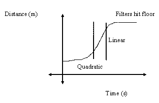
Figure 2 shows qualitatively what a graph of distance vs. time might
look like. Initially the distance grows quadratically in time, but as the terminal velocity is
approached, the distance tends to grow linearly in time. The slope of the linear portion of the
distance versus time graph is the terminal velocity. We wish to extract this slope and thus obtain
the terminal velocity.
Figure 2 Schematic of “Typical” Data
Click on
the Position vs. time graph so that it is active. Click and drag over the region of the data
that appears to be linear. Click on the linear fit button (looks like a
tangent line with the letter R on it).
This will automatically give you the best fit line and put the equation
of the best fit line in a tiny box on the screen. Record the mass of the stack of filters and
the terminal velocity in the data table below.
Figure 3 Data Table
|
Trial |
Mass (kg) |
Terminal Velocity (m/s) |
|
1 |
|
|
|
2 |
|
|
|
3 |
|
|
|
4 |
|
|
|
5 |
|
|
Q8. Sketch a
graph of velocity vs. time in the space below.
Q9. Indicate
on the graph the region where terminal velocity was reached. What feature of the graph tells you that
terminal velocity was reached?
Q10. Sketch a
graph of acceleration vs. time in the space below.
Q11. Indicate
on the graph the region where terminal velocity was reached. What feature of the graph tells you that
terminal velocity was reached?
3. Repeat the
Experiment for Different Masses
Repeat
your series of measurements four more times, each time increasing the number of
coffee filters by 1. Each trial, record
the mass of the coffee filters and the terminal velocity you obtained in the
data table.
Data Analysis
The
information we wish to extract from our data is which of the models for air
resistance better describes the data.
The linear model for air resistance gives a result where the terminal
velocity is a linear function of the mass, and the quadratic model yields a
terminal velocity which is proportional to the square root of the mass. In either case, we expect a result of the
form v = kmn (1) where k is some constant
and n is some power. We wish to
determine the exponent.
Q13. List the
value of the exponent for the linear case
n =
Q14. List the
value of the exponent for the quadratic case
n =
A common
data analysis tool to extract information about exponents is to plot a log-log
plot. In a log-log plot instead of plotting y vs. x we plot log(y) vs.
log(x). The log can be to any base, but
typically base 10 is chosen. If we
consider v = kmn (1), let us examine what happens when we
take the log of both sides. Remember the
important properties of logarithms i) log(AB) = log(A) + log(B) and ii) log(An) = n log(A).
Q15. Take the
log of both sides of (1) and use the properties of the logarithms to obtain an
expression for log(v) in terms of log(m), n and log(k)
Q16. Based on
your answer to Q15 what type of graph should you obtain if you graph log(v) vs. log(m).
Q17. What
will be the slope of the graph of log(v) vs. log(m) if
the linear air resistance model is a better description of this experiment?
Q18. What will be the slope of the graph of log(v) vs. log(m) if the quadratic air resistance model is a
better description of this experiment?
Use LoggerPro or Excel to graph log(v)
vs. log(m) and perform a linear regression analysis to determine the
slope.
Q19. Record
your slope
Q20. Is your
slope consistent with either of the models discussed in this lab? Explain your answer.
Q21. Attach a copy of your log-log plot to the
handout.
Further Analysis
In this part we will find an analytical
expression for the position as a function of time for the case of linear air
resistance. In Q2 we should have written
![]() (2)
.
(2)
.
Q22. To see this, divide both sides of (2) by (mg
– bv)m.
Q23. The next step in solving by separation of
variables is multiplying both sides by dt. Carry this out.
Q24. Part of the term on the left should look like
dv/dt dt. What does this equal? Replace it in the answer to Q23.
Q25. Now integrate both sides of Q24.
Don't forget that you will need an arbitrary constant. Hint: ![]()
Q26. Solve the expression you obtained in Q25 for
v. Evaluate the constant by using that v(0) = 0.
Q27. You should notice that your answer involves
an exponential function. The terminal
velocity can be found by considering the limit at t →∞. Take ![]() . Do you get the same
result as you found in Q5?
. Do you get the same
result as you found in Q5?