The basics

Sometimes, the coordinate system you need to use to work an integral is fairly obvious.  As an example, consider finding given integral over the region between the following sets of curves:

x ydA where D is the region between the graphs of:
    3x-y=1, y=3x-6,x y=1, and x y=2 in the first quadrant.

If you think about it, this is really the region:

    1≤3x-y≤6 and 1≤x y≤ 2

which looks like:

Now, you could do this using 3 separate integrals.  However, by using a change of coordinates, with u=3x-y and v=x y, you could work it using a single integral.  So, let's set this up as a change of coordinates.  I'm going to define two transformation:

XYtoUV:→ maps from D→ (takes an input of {x,y} and returns a point in {u,v})
UVtoXY:→ maps from →D (takes an input of {u,v} and returns a point in {x,y})

(Remember that you take the Jacobian of UVtoXY; in the notation we use in class, XYtoUV would be and UVtoXY would be T.)

This says u=3x-y and v=x y.  Now, the function we want to integrate:

Now, in order to find T(UVtoXY), we need to solve the system of equations for x and y (in terms of u and v).  We can do this with the solve command:

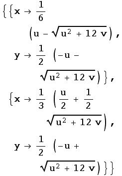
Notice that I gave the solution set a name (solveInverse), so I can refer back to it.  Also, notice that there are two sets of solutions.  Should this be a surprise?  (Hint:  Check out the graph earlier...)  If you look at these carefully, you will see that the second set is the one in the first quadrant (for u and v in the ranges we nned).

Further, notice that the solutions are not given in the form {x=blah,y=bleh}, they are given in the form {x→blah,y→bleh}.  These are called "replacement rules", which means that they are a set of instructions ("replace x with blah and replace y with bleh").  We can use the "replace all" operator /. to apply the rules.  So, for example, the following code:

replaces all the x's in the expression +2x-y with x=3.  So, we could assign these solutions to set up our UVtoXY function as follows:

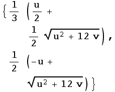
This replaces {x,y} with the solutions we found above (called solveInverse).  Since we only wanted the solution in the first quadrant (the second one), we used solveInverse[[2]].

Now, we also need the Jacobian determinant.  In Mathematica, you can find the Jacobian of a function by:

D[function[var1,var2,va3,...],{{var1,var2,va3,...}}]

(Notice the double {]'s enclosing the variables.  So, for example:

Or, to make it look cooler:

We then need to take the determinant; so, here we can do the following:

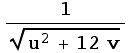
(I use the //FullSimplify at the end of the line to make sure Mathematica has simplified it as much as possible before I go on.)  Notice, this will always be positive, so I don't need to take the absolute value.

Now, we need to take the composition of f and our transform T, i.e., f(T(u,v)):

(Just a kindly word of warning here:  In this problem, f(T(u,v)) simplified out really nicely.  However, it is often the case that it will be much more complicated than f(x,y) was.  If it is too complicated, the transformed integral may be too hard for Mathematica to solve and you may have to go back and try something else...)

Finally, pull it all together:

You could certainly combine several of these steps together, but hopefully this gives you an idea how to work your way through one of these.  If you really want to, you could do the integral without using the fUV and detJ expressions:

(The real problem with this is that you don't explicitly see what the determinant of the Jacobian looks like, so you don't really know whether you have the right sign for the Jacobian determinant.  If it is negative everywhere, then your answer will only be off by a sign, but if it is negative in some parts of your domain and positive in others, you have a much bigger problem.)

Created by Mathematica  (April 3, 2007)